Stat-Ease Blog

Categories
Mixture Designs – Gimmick or Magic?
Years ago, I attended Stat-Ease’s Modern DOE workshop in Minneapolis—a five day deep dive into factorial and response surface methods (RSM). I then completed a four day course on Mixture Design for Optimal Formulations. Since then, I’ve trained practitioners and coached users through hundreds of experiments. One pattern is consistent: most people—myself included—gravitate toward familiar factorial or RSM designs and hesitate to use mixture designs for formulation work.
The result is force-fitting RSM tools onto mixture problems. Like using a flathead screwdriver on a Phillips screw, it can work, but it’s rarely ideal. And, avoiding mixture designs can actually create real problems. So, what makes mixtures unique, and what goes wrong when we ignore that?
Why Mixtures Are Different
In mixtures, ratios drive responses, not absolute amounts. The flavor of a cookie depends on the ratio of flour, sugar, fat, and salt; not the grams of sugar alone. And because mixture components must sum to a total (often 100%), choosing levels for some ingredients automatically constrains the rest.
The Ratio Workaround—and Its Limits
A common workaround is to convert a q-component mixture into q-1 ratios and run a standard RSM design¹. For example, suppose we’re formulating a sweetener blend (A = sugar, B = corn syrup, C = honey) that always makes up 10% of a cookie recipe. If we express the system using ratios B:A and C:A, we can build a two factor RSM design with ratio levels like 1:1, 2:1, and 3:1.
But compared to a true three component mixture design, the difference is clear. The ratio based design samples only narrow rays of the mixture space, leaving large regions unexplored. Standard error plots show that a proper mixture design provides far better prediction capability across the full region.
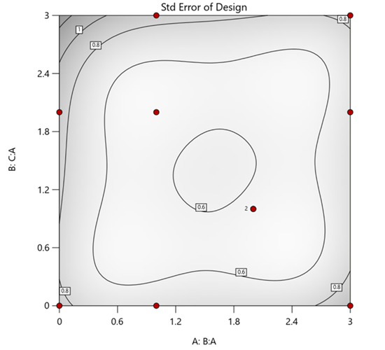
Figure 1. Optimal 10-run RSM design layout using two ratios for a three-component mixture. The shading conveys the relative standard error: lighter is lower, darker is higher.
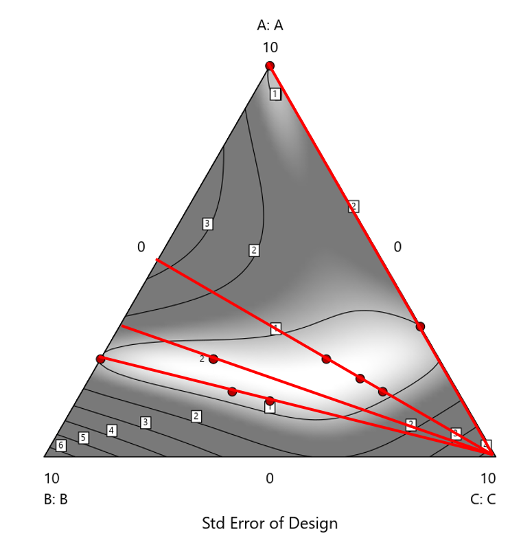
Figure 2. Translation of the ratio design from Figure 1 onto a three-component layout.
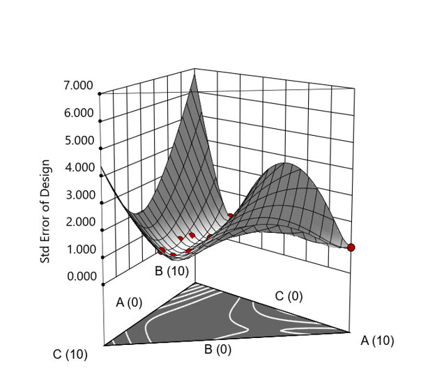
Figure 3. Standard error 3D plot of the 10-run ratio design.
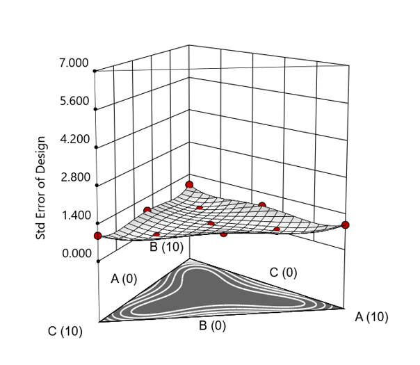
Figure 4. Standard error 3D plot for a 10-run augmented simplex mixture design.
In short: the ratio trick can work, but it never matches the statistical properties of a proper mixture design.
The Slack Component Argument
Another justification for using RSM is when one ingredient is believed to be inconsequential. Perhaps the component is believed to be inert or is simply a diluent that makes up the balance of a formulation. The idea is to treat this component as a slack variable and allow it to fill whatever space remains after setting the other ingredients. One slack approach is to simply use the upper and lower values as levels of the non slack components in a standard RSM. Below is a comparison of a three-component system analyzed as a true mixture design alongside a two-factor RSM that eliminates the diluent as a component.
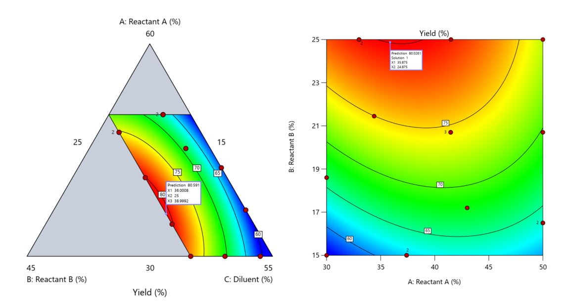
Figure 5. Optimization comparison of a three component mixture design and a two factor (component) RSM approach
In this case, both approaches found essentially the same optimal conditions. Ignoring the diluent really didn’t impact the story, but the RSM approach is not specifically assessing the interactive behavior between the reactants and the diluent. If we study the system as an RSM, we assume the interactions involving the omitted component were not consequential—which may not be true. Cornell² states that the factor effects we are seeing are actually the effects confounded with the opposite effect of the ignored component. Without using a mixture design, we would have no way of validating our assumptions about these interactions.
Cornell³ also describes an alternative slack approach where the slack component is included in the design but excluded from the predictive model. Some practitioners believe this approach makes sense when the diluent interacts weakly with the key ingredients, the omitted component is the one with the widest range of proportionate values, or if that component makes up the bulk of the formulation. But statistically, this presents some interesting complexities.
Using the above chemical reaction example, Figure 6 shows the model differences between the Scheffé approach and the resulting models when each component is considered the slack component.
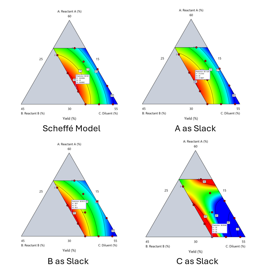
Figure 6. Comparing the Scheffé and Slack modeling techniques.
Note that in this example, while some of the models are similar, the one involving the diluent as the slack variable differs most from the Scheffé standard. Had we assumed the diluent could have been used as the slack variable, we would have poorly modeled and optimized the system.
Because slack variable models exclude at least one component and its interactions, they’re best avoided when possible.
When Components Don’t Share a Scale
Mixture designs require all components to share a common basis (percent, ppm, etc.). This becomes awkward when ingredients span vastly different scales—for example, large amounts of reactants plus a catalyst at ppm levels. The phenomenon is often called the “sliver effect” because the design space becomes a very narrow region for the low-level component, as shown in Figure 7.
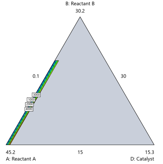
Figure 7. The sliver effect that can occur when one component is present in much lower levels than the balance of the formulation.
One way to avoid a sliver is to change the metric: in this case, changing to molar percent may put the components on a comparable basis and all components could have been included in the mixture design. Or, if I’m still avoiding mixtures, a practical solution is a combined design: treat the main ingredients as a mixture and the catalyst as a process variable. Both the mixture and the catalyst should be modeled quadratically to capture interactions. However, the interactive nature of components is best resolved when all ingredients are included in the mixture design.
The Bottom Line
For formulations, and recipes, the best results come from designs built specifically for mixtures. They’re not gimmicks or magic; they’re the right tools for the job. Stat-Ease provides tutorials and webinars to help you get started:
- A Crash Course in Mixture Design of Experiments
- Optimal experiment designs that combine mixture, process and categorical inputs
Or, if you’d prefer a hands-on, instructor-led experience (maybe with me!), sign up for one of the following courses:
References:
- Response Surface Methodology, 4th edition, Myers, Montgomery, Anderson-Cook, pp. 759-763 (Wiley).
- Experiments with Mixtures, 3rd edition, John Cornell, p. 16 (Wiley).
- Experiments with Mixtures, 3rd edition, John Cornell, p. 333-343 (Wiley).
Like the blog? Never miss a post - sign up for our blog post mailing list.
Ask An Expert: Jay Davies
Next in our 40th anniversary “Ask an Expert” blog series is John "Jay" Davies, who's an absolute rock star when it comes to teaching and implementing DOE. He's lent us his expertise before - see this talk from our 2022 Online DOE Summit - and he shared an anecdote with our statistical experts about how he approaches switching to DOE methods when working with new groups in the Army. He kindly agreed to let us publish it as part of this series.
For the past 14 years, I’ve been a Research Physicist with the U.S. Army DEVCOM Chemical Biological Center at Aberdeen Proving Grounds, MD as a member of the Decontamination Sciences Branch, which specializes in developing techniques/chemistries to neutralize chemical warfare agents. I’m dedicated to applied statistical analysis ranging from multi-laboratory precision studies to design of experiments (DOE). The Decontamination Sciences Branch has been integrating DOE methods into many of their chemical agent decontamination research programs.
I’m happy to report that the DOE methods here at the Chemical Biological Center are really catching on. I collaborated on 24 DOEs from 2014 through 2021. Then, in 2021-22, we completed 26 DOEs across 10 different programs. I’ve been doing a lot of mixture-process DOEs with the Bio Sciences groups for synthetic biology and bio manufacturing applications, and once the other groups saw the information that we were getting from just a single day’s worth of data, they too wanted to try DOE.
Lately, I’ve changed the formula that I use for the initial consultations when visiting a group that has expressed an interest in DOE but has never used DOE before. Previously we’d go right into their project, and I’d tell them how we might construct a DOE for their application. However, I’ve found that it’s too much of a culture shock if we go right into talking about what a DOE for their application might look like. Instead, especially if I’m working with a group that has no DOE experience at all, I now devote about 1 hour to discuss DOE methods in general before we even mention their actual application. In this discussion, I reveal the major differences that they are going to see with a DOE, which are:
- We’re not going to replicate every sample, we may even have zero exact replication.
- We’re not going to test every possible combination of factors.
- Sample sizes are going to be 70% to 95% smaller than what they are used to doing.
- We are not going to change “one factor at a time”, in fact we’ll be changing all factors at once.
- The designs might look chaotic, but they are strategically created to contain a hidden orthogonal structure, along with hidden replication, that is not apparent.
- You will see that many of the DOE samples contain factor combinations that don’t seem to make sense. This is because each sample is not designed as a stand-alone shot at optimization. Rather, the samples cumulatively are working in concert to tease out the influences of each factor. This will let us fit a predictive model that we will then use to predict the optimal settings of factors.
Recently, I was following this format with a group that had never used DOE before. We had a great back-and-forth dialog as I went through the bullets above and explained a bit about each point. They asked many questions and were really following along. Then, after about an hour we got into their application and I just sketched out a prototype quadratic mixture-process DOE that I thought would give them a good idea of what the initial DOE might look like, with 30 samples in total. I then went over what some simulated outputs for the DOE generated prediction model might look like. At this point one of them stopped me and with a very perplexed look on his face, said “hold on, hold on…wait a minute here. Are you telling us that if we run just those 30 samples, we would be able to predict the optimal formulation and the optimal process setting for this system?“
This scientist had been following along, asking questions and really absorbing the information in the past hour as we walked through the DOE basics, but I could see that at that moment things were just sinking in. He realized the ramifications of what we had just discussed – typically, this group might have had to run several hundreds of samples to characterize similar systems, but with DOE they would only need about 30 samples. I responded to his question saying, “Yes that’s exactly what I’m telling you. We’ve run dozens of these mixture-process DOEs, many of them much more complex than this system, and they do work.” This individual, a mid-career researcher, then responded, “How is it possible that we have not heard of this stuff before?” I told him, “I can’t give you a good answer to that one.”
And there you have it! Let us know if you want to talk about saving time & money with DOE: our statistical experts and first-in-class software make it easier than ever.
DISTRIBUTION STATEMENT A. Approved for Public Release: Distribution is Unlimited
Randomization Done Right
Randomization is essential for success with planned experimentation (DOE) to protect factor effects against bias by lurking variables. For example, consider the 8-run, two-level factorial design shown in Table 1. It lays out the low (−) and high (+) coded levels of each factor in standard, not random, order. Notice that factor C changes level only once throughout the experiment—first being set at the low (minus) level for four runs, followed by the remaining four runs set at the high (plus) level. Now, let’s say that the humidity in the room increases throughout the day—affecting the measured response. Since the DOE runs are not randomized, the change in humidity biases the calculated effect of the non-randomized factor C. Therefore, the effect of factor C includes the humidity change – it is no longer purely due to the change from low to high. This will cause analysis problems!
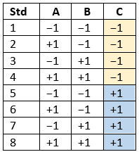
Table 1: Standard order of 8-run design
Randomization itself presents some problems. For example, one possible random order is the classic standard layout, which, as you now know, does not protect against time-related effects. If this unlikely pattern, or other non-desirable patterns are seen, then you should re-randomize the runs to reduce the possibility of bias from lurking variables.
Randomizing center points or other replicates
Replicates, such as center points, are used to collect information on the pure error of the system. To optimize the validity of this information, center points should be spaced out over the experimental run order. Random order may inadvertently place replicates in sequential order. This requires manual intervention by the researcher to break up or separate the repeated runs so that each run is completed independently of the matching run.
In both Design-Expert® software and Stat-Ease 360 you can re-randomize by right-clicking on the Run column header and selecting Randomize, as shown in Figure 1. You can also simply edit the Run order and swap two runs by changing the run numbers manually. This is often the easiest method when you want to separate center points, for example.
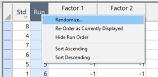
Figure 1: Right-click to Randomize
When Randomization Doesn’t Work
While randomization is ideal statistically, sometimes it is cumbersome in practice. For instance, temperature can take a very long time to change, so completely randomizing the runs may cause the experiment to go way beyond the time budget. In this case, researchers look for ways to reduce the complete randomization of the design.
I want to highlight a common DOE mistake. An incorrect way to restrict the randomization is to use blocks. Blocking is a statistical technique that groups the experimental runs to eliminate a potential source of variation from the data analysis. A common blocking factor is “day”, setting the block groups to eliminate day-to-day variation. Although this is a form of restricting randomization, if you block on an experimental factor like temperature, then statistically the block (temperature) effect will be removed from the analysis. Any interaction effect with that block will also be removed. The removal of this key effect very likely destroys the entire analysis! Blocking is not a useful method for restricting the randomization of a factor that is being studied in the experiment. For more information on why you would block, see “Blocking: Mowing the Grass in Your Experimental Backyard”.
If factor changes need to be restricted (not fully randomized), then building a split-plot design is the best way to go. A split-plot design takes into account the hard-to-change versus easy-to-change factors in a restricted randomization test plan. Perfect! The associated analysis properly assesses the differences in variation between these two groups of factors and provides the correct effect evaluation. The statistical analysis is a bit more complex, but good DOE software will handle it easily. Split-plot designs are a more complex topic, but commonly used in today’s experimental practices. Learn more about split-plot designs in this YouTube video: Split Plot Pros and Cons – Dealing with a Hard-to-Change Factor.
Wrapping up
Randomization is essential for valid and unbiased factor effect calculations, which is central to effective design of experiments analysis. It is up to the experimenter to ensure that the randomization of the experimental runs meets the DOE goals. Manual intervention may be required to separate any replicated points, such as center points. If complete randomization is not possible from a practical standpoint, build a split-plot design that statistically accounts for those restrictions.